JSOES Bongo Data Exploratory Analysis
Markus Min
2025-05-27
This page contains exploratory analysis for the Bongo net data from JSOES. Please note that because the Bongo net tows occur during daylight hours, the tow composition is biased towards taxa/life stages that do not vertically migrate. While different life stages of some species are counted separately for this data, for this exploratory analysis we summed abundances across life stages.
In this document, I will characterize general patterns in this dataset, and then visualize some key groups of salmon forage that are caught in this survey. This document also contains the scripts to export these groups, formatted for inclusion in the model.
Data Overview
We will first explore the most common and most abundant taxa in this dataset.
| genus_species | common_name | mean_density_per_m3 | sd_density_per_m3 |
|---|---|---|---|
| Euphausiidae | Euphausiidae | 117.5 | 703.9 |
| Cirripedia | Barnacles | 34.8 | 757.1 |
| Chaetognatha | Chaetognatha | 3.5 | 16.1 |
| Euphausia pacifica | Euphausia Pacifica | 3.5 | 29.4 |
| Mitrocoma cellularia | Mitrocoma Cellularia (Cross Jellyfish) | 3.4 | 29.9 |
| Limacina | Limacina | 3.0 | 23.3 |
| 22 division fish egg | 22 Division Fish Egg | 2.9 | 8.6 |
| Engraulis mordax | Northern Anchovy | 2.5 | 25.1 |
| Calanus marshallae | Calanus Marshallae | 2.4 | 11.8 |
| Neotrypaea californiensis | Bay Ghost Shrimp | 2.4 | 159.8 |
| genus_species | common_name | prop_samples |
|---|---|---|
| Euphausia pacifica | Euphausia Pacifica | 0.83 |
| Euphausiidae | Euphausiidae | 0.80 |
| Thysanoessa spinifera | Thysanoessa Spinifera | 0.76 |
| Calanus marshallae | Calanus Marshallae | 0.70 |
| Cancer oregonensis/productus | Cancer Oregonensis/Productus | 0.70 |
| Chaetognatha | Chaetognatha | 0.70 |
| Themisto pacifica | Themisto Pacifica | 0.66 |
| Cirripedia | Barnacles | 0.64 |
| Limacina | Limacina | 0.49 |
| Crangonidae | Crangon | 0.46 |
Annual time series
This Shiny app can be used to explore the abundances of different taxa across the full length of the time series. In this Shiny app, I take the mean log density across the survey region to create a simple index of abundance.
Exploring broad groups of taxa
The JSOES bongo data contains data on both the direct prey of Pacific salmon as well as the prey items of the prey of Pacific salmon. The direct salmon prey that is caught in this survey includes Euphausiids, Cancer crab larvae, hyperiid amphipods, and non-cancer crab larvae. The abundance of copepods has also been correlated with salmon marine survival, and as such we will also examine these taxa.
Let’s ID everything that’s seen in at least 0.5% of samples. This accounts for 118 of 215 total taxa identified in this survey.
Plotting distributions of some common taxa
Let’s visualize the following groups for our study, since they are known direct prey items of salmon:
- Cancer crab larvae
- Non-cancer crab larvae
- shrimp larvae
- Hyperiid amphipods
Krill are also consumed by salmon, but we have other surveys that provide better estimates of krill abundance.


Lower trophic levels
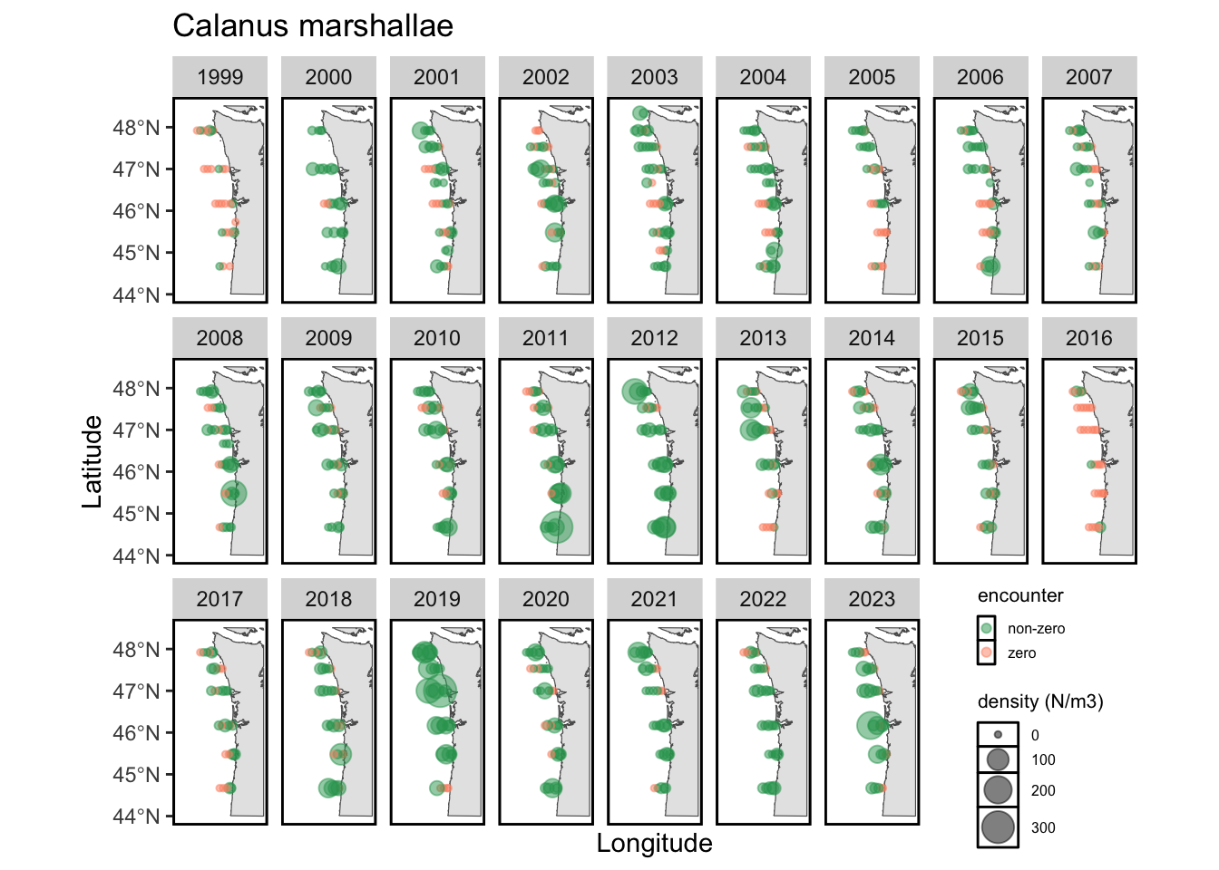
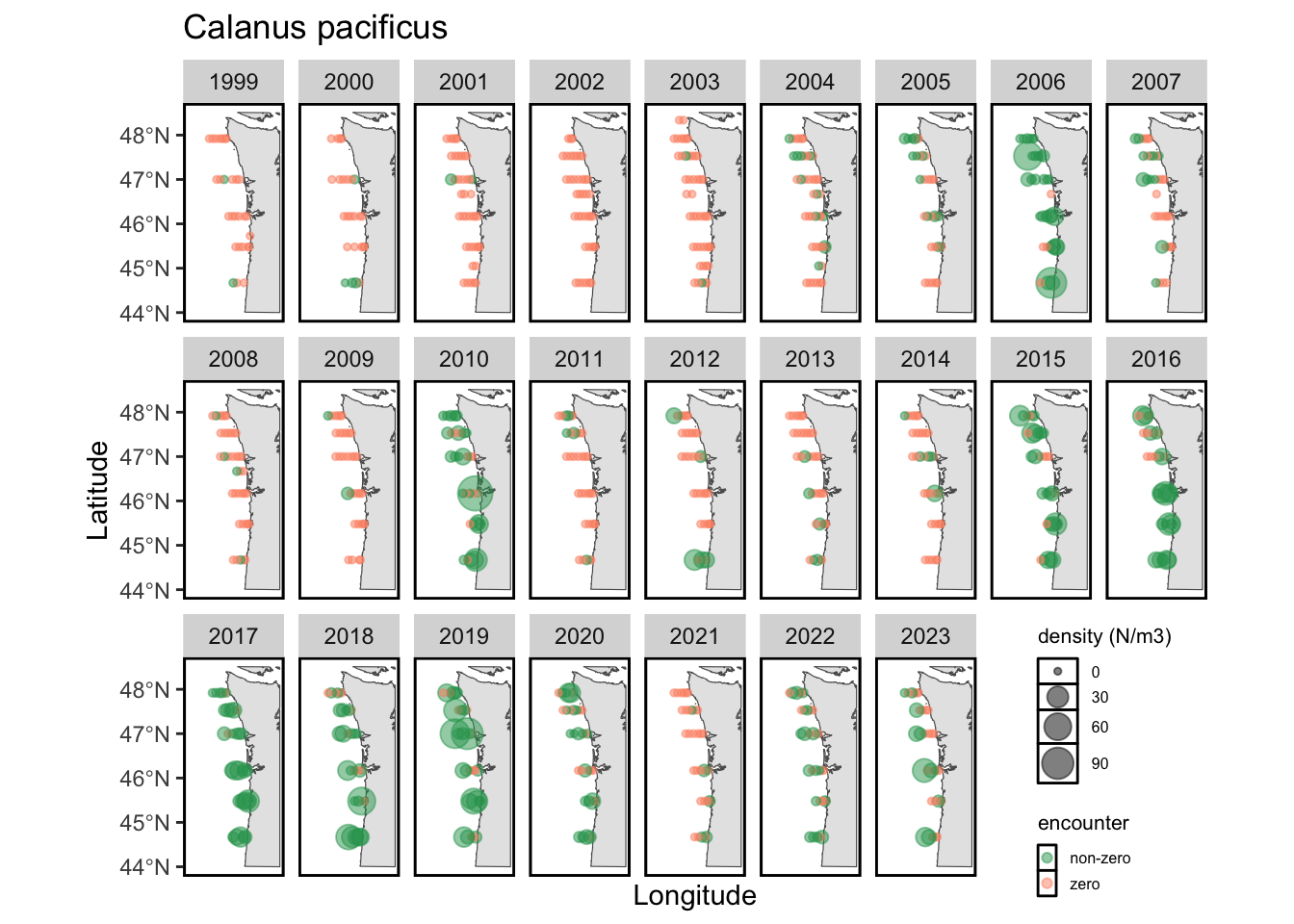
While we visualize the direct forage of juvenile salmon above, the Bongo data also helps us characterize the distributions and abundance of taxa that are 2+ trophic levels below salmon (i.e., the prey of salmon prey). The literature suggests that the most important of these are copepods, as the abundance of cold-water vs. warm-water copepods has been linked with marine survival. Below, I provide static maps of two focal taxa for this survey: Calanus marshallae (an abundant cold-water copepod) and Calanus pacificus (an abundant warm-water coepod).
Export data
In the last section of this script, we will export the following functional groups for inclusion in spatiotemporal models. The data will be formatted with the total density of each functional group at each station.
- Cancer crab larvae
- Non-cancer crab larvae
- shrimp larvae
- Hyperiid amphipods